Monday, December 17, 2018

PyPy Winter Sprint Feb 4-9 in Düsseldorf

 PyPy Sprint February 4th-9th 2019 in Düsseldorf


The next PyPy sprint will be held in the Computer Science department of Heinrich-Heine Universität Düsseldorf from the 4th to the 9st of February 2019 (nine years after the last sprint there). This is a fully public sprint, everyone is welcome to join us.

Topics and goals

  • improve Python 3.6 support
  • discuss benchmarking situation
  • progress on utf-8 branches
  • cpyext performance and completeness
  • packaging: are we ready to upload to PyPI?
    • issue 2617  - we expose too many functions from lib-pypy.so
    • manylinux2010 - will it solve our build issues?
    • formulate an ABI name and upgrade policy
  • memoryview(ctypes.Structure) does not create the correct format string
  • discussing the state and future of PyPy and the wider Python ecosystem

Location

The sprint will take place in seminar room 25.12.02.55 of the computer science department.  It is in the building 25.12 of the university campus, second floor. Travel instructions

Exact times

Work days: starting February 4th (10:00), ending February 9th (~afternoon). The break day will probably be Thursday.

Registration


Please register by Mercurial::
https://bitbucket.org/pypy/extradoc/
https://bitbucket.org/pypy/extradoc/src/extradoc/sprintinfo/ddorf2019/people.txt

or on the pypy-dev mailing list if you do not yet have check-in rights:

Looking forward to seeing everyone there!

Thursday, November 29, 2018

Funding for 64-bit Armv8-a support in PyPy

Hello everyone

At PyPy we are trying to support a relatively wide range of platforms. We have PyPy working on OS X, Windows and various flavors of linux (and unofficially various flavors of BSD) on the software side, with hardware side having x86, x86_64, PPC, 32-bit Arm (v7) and even zarch. This is harder than for other projects, since PyPy emits assembler on the fly from the just in time compiler and it requires significant amount of work to port it to a new platform.

We are pleased to inform that Arm Limited, together with Crossbar.io GmbH, are sponsoring the development of 64-bit Armv8-a architecture support through Baroque Software OU, which would allow PyPy to run on a new variety of low-power, high-density servers with that architecture. We believe this will be beneficial for the funders, for the PyPy project as well as to the wider community.

The work will commence soon and will be done some time early next year with expected speedups either comparable to x86 speedups or, if our current experience with ARM holds, more significant than x86 speedups.

Best,
Maciej Fijalkowski and the PyPy team


Thursday, November 15, 2018

Guest Post: Implementing a Calculator REPL in RPython

This is a tutorial style post that walks through using the RPython translation toolchain to create a REPL that executes basic math expressions.

We will do that by scanning the user's input into tokens, compiling those tokens into bytecode and running that bytecode in our own virtual machine. Don't worry if that sounds horribly complicated, we are going to explain it step by step.

This post is a bit of a diversion while on my journey to create a compliant lox implementation using the RPython translation toolchain. The majority of this work is a direct RPython translation of the low level C guide from Bob Nystrom (@munificentbob) in the excellent book craftinginterpreters.com specifically the chapters 14 – 17.

The road ahead

As this post is rather long I'll break it into a few major sections. In each section we will have something that translates with RPython, and at the end it all comes together.

A REPL

So if you're a Python programmer you might be thinking this is pretty trivial right?

I mean if we ignore input errors, injection attacks etc couldn't we just do something like this:

"""
A pure python REPL that can parse simple math expressions
"""
while True:
    print(eval(raw_input("> ")))

Well it does appear to do the trick:

$ python2 section-1-repl/main.py
> 3 + 4 * ((1.0/(2 * 3 * 4)) + (1.0/(4 * 5 * 6)) - (1.0/(6 * 7 * 8)))
3.1880952381

So can we just ask RPython to translate this into a binary that runs magically faster?

Let's see what happens. We need to add two functions for RPython to get its bearings (entry_point and target) and call the file targetXXX:

targetrepl1.py

def repl():
    while True:
        print eval(raw_input('> '))


def entry_point(argv):
    repl()
    return 0


def target(driver, *args):
    return entry_point, None

Which at translation time gives us this admonishment that accurately tells us we are trying to call a Python built-in raw_input that is unfortunately not valid RPython.

$ rpython ./section-1-repl/targetrepl1.py
...SNIP...
[translation:ERROR] AnnotatorError: 

object with a __call__ is not RPython: <built-in function raw_input>
Processing block:
 block@18 is a <class 'rpython.flowspace.flowcontext.SpamBlock'> 
 in (target1:2)repl 
 containing the following operations: 
       v0 = simple_call((builtin_function raw_input), ('> ')) 
       v1 = simple_call((builtin_function eval), v0) 
       v2 = str(v1) 
       v3 = simple_call((function rpython_print_item), v2) 
       v4 = simple_call((function rpython_print_newline)) 

Ok so we can't use raw_input or eval but that doesn't faze us. Let's get the input from a stdin stream and just print it out (no evaluation).

targetrepl2.py

from rpython.rlib import rfile

LINE_BUFFER_LENGTH = 1024


def repl(stdin):
    while True:
        print "> ",
        line = stdin.readline(LINE_BUFFER_LENGTH)
        print line


def entry_point(argv):
    stdin, stdout, stderr = rfile.create_stdio()
    try:
        repl(stdin)
    except:
        return 0


def target(driver, *args):
    return entry_point, None

Translate targetrepl2.py – we can add an optimization level if we are so inclined:

$ rpython --opt=2 section-1-repl/targetrepl2.py
...SNIP...
[Timer] Timings:
[Timer] annotate                       ---  1.2 s
[Timer] rtype_lltype                   ---  0.9 s
[Timer] backendopt_lltype              ---  0.6 s
[Timer] stackcheckinsertion_lltype     ---  0.0 s
[Timer] database_c                     --- 15.0 s
[Timer] source_c                       ---  1.6 s
[Timer] compile_c                      ---  1.9 s
[Timer] =========================================
[Timer] Total:                         --- 21.2 s

No errors!? Let's try it out:

$ ./target2-c 
1 + 2
>  1 + 2

^C

Ahh our first success – let's quickly deal with the flushing fail by using the stdout stream directly as well. Let's print out the input in quotes:

from rpython.rlib import rfile

LINE_BUFFER_LENGTH = 1024


def repl(stdin, stdout):
    while True:
        stdout.write("> ")
        line = stdin.readline(LINE_BUFFER_LENGTH)
        print '"%s"' % line.strip()


def entry_point(argv):
    stdin, stdout, stderr = rfile.create_stdio()
    try:
        repl(stdin, stdout)
    except:
        pass
    return 0


def target(driver, *args):
    return entry_point, None

Translation works, and the test run too:

$ ./target3-c 
> hello this seems better
"hello this seems better"
> ^C

So we are in a good place with taking user input and printing output... What about the whole math evaluation thing we were promised? For that we are can probably leave our RPython REPL behind for a while and connect it up at the end.

A virtual machine

A virtual machine is the execution engine of our basic math interpreter. It will be very simple, only able to do simple tasks like addition. I won't go into any depth to describe why we want a virtual machine, but it is worth noting that many languages including Java and Python make this decision to compile to an intermediate bytecode representation and then execute that with a virtual machine. Alternatives are compiling directly to native machine code like (earlier versions of) the V8 JavaScript engine, or at the other end of the spectrum executing an abstract syntax tree – which is what the Truffle approach to building VMs is based on.

We are going to keep things very simple. We will have a stack where we can push and pop values, we will only support floats, and our VM will only implement a few very basic operations.

OpCodes

In fact our entire instruction set is:

OP_CONSTANT
OP_RETURN
OP_NEGATE
OP_ADD
OP_SUBTRACT
OP_MULTIPLY
OP_DIVIDE

Since we are targeting RPython we can't use the nice enum module from the Python standard library, so instead we just define a simple class with class attributes.

We should start to get organized, so we will create a new file opcodes.py and add this:

class OpCode:
    OP_CONSTANT = 0
    OP_RETURN = 1
    OP_NEGATE = 2
    OP_ADD = 3
    OP_SUBTRACT = 4
    OP_MULTIPLY = 5
    OP_DIVIDE = 6

Chunks

To start with we need to get some infrastructure in place before we write the VM engine.

Following craftinginterpreters.com we start with a Chunk object which will represent our bytecode. In RPython we have access to Python-esq lists so our code object will just be a list of OpCode values – which are just integers. A list of ints, couldn't get much simpler.

section-2-vm/chunk.py

class Chunk:
    code = None

    def __init__(self):
        self.code = []

    def write_chunk(self, byte):
        self.code.append(byte)

    def disassemble(self, name):
        print "== %s ==\n" % name
        i = 0
        while i < len(self.code):
            i = disassemble_instruction(self, i)

From here on I'll only present minimal snippets of code instead of the whole lot, but I'll link to the repository with the complete example code. For example the various debugging including disassemble_instruction isn't particularly interesting to include verbatim. See the github repo for full details

We need to check that we can create a chunk and disassemble it. The quickest way to do this is to use Python during development and debugging then every so often try to translate it.

Getting the disassemble part through the RPython translator was a hurdle for me as I quickly found that many str methods such as format are not supported, and only very basic % based formatting is supported. I ended up creating helper functions for string manipulation such as:

def leftpad_string(string, width, char=" "):
    l = len(string)
    if l > width:
        return string
    return char * (width - l) + string

Let's write a new entry_point that creates and disassembles a chunk of bytecode. We can set the target output name to vm1 at the same time:

targetvm1.py

def entry_point(argv):
    bytecode = Chunk()
    bytecode.write_chunk(OpCode.OP_ADD)
    bytecode.write_chunk(OpCode.OP_RETURN)
    bytecode.disassemble("hello world")
    return 0

def target(driver, *args):
    driver.exe_name = "vm1"
    return entry_point, None

Running this isn't going to be terribly interesting, but it is always nice to know that it is doing what you expect:

$ ./vm1 
== hello world ==

0000 OP_ADD       
0001 OP_RETURN    

Chunks of data

Ref: http://www.craftinginterpreters.com/chunks-of-bytecode.html#constants

So our bytecode is missing a very crucial element – the values to operate on!

As with the bytecode we can store these constant values as part of the chunk directly in a list. Each chunk will therefore have a constant data component, and a code component.

Edit the chunk.py file and add the new instance attribute constants as an empty list, and a new method add_constant.

    def add_constant(self, value):
        self.constants.append(value)
        return len(self.constants) - 1

Now to use this new capability we can modify our example chunk to write in some constants before the OP_ADD:

    bytecode = Chunk()
    constant = bytecode.add_constant(1.0)
    bytecode.write_chunk(OpCode.OP_CONSTANT)
    bytecode.write_chunk(constant)

    constant = bytecode.add_constant(2.0)
    bytecode.write_chunk(OpCode.OP_CONSTANT)
    bytecode.write_chunk(constant)

    bytecode.write_chunk(OpCode.OP_ADD)
    bytecode.write_chunk(OpCode.OP_RETURN)

    bytecode.disassemble("adding constants")

Which still translates with RPython and when run gives us the following disassembled bytecode:

== adding constants ==

0000 OP_CONSTANT  (00)        '1'
0002 OP_CONSTANT  (01)        '2'
0004 OP_ADD       
0005 OP_RETURN

We won't go down the route of serializing the bytecode to disk, but this bytecode chunk (including the constant data) could be saved and executed on our VM later – like a Java .class file. Instead we will pass the bytecode directly to our VM after we've created it during the compilation process.

Emulation

So those four instructions of bytecode combined with the constant value mapping 00 -> 1.0 and 01 -> 2.0 describes individual steps for our virtual machine to execute. One major point in favor of defining our own bytecode is we can design it to be really simple to execute – this makes the VM really easy to implement.

As I mentioned earlier this virtual machine will have a stack, so let's begin with that. Now the stack is going to be a busy little beast – as our VM takes instructions like OP_ADD it will pop off the top two values from the stack, and push the result of adding them together back onto the stack. Although dynamically resizing Python lists are marvelous, they can be a little slow. RPython can take advantage of a constant sized list which doesn't make our code much more complicated.

To do this we will define a constant sized list and track the stack_top directly. Note how we can give the RPython translator hints by adding assertions about the state that the stack_top will be in.

class VM(object):
    STACK_MAX_SIZE = 256
    stack = None
    stack_top = 0

    def __init__(self):
        self._reset_stack()

    def _reset_stack(self):
        self.stack = [0] * self.STACK_MAX_SIZE
        self.stack_top = 0

    def _stack_push(self, value):
        assert self.stack_top < self.STACK_MAX_SIZE
        self.stack[self.stack_top] = value
        self.stack_top += 1

    def _stack_pop(self):
        assert self.stack_top >= 0
        self.stack_top -= 1
        return self.stack[self.stack_top]

    def _print_stack(self):
        print "         ",
        if self.stack_top <= 0:
            print "[]",
        else:
            for i in range(self.stack_top):
                print "[ %s ]" % self.stack[i],
        print

Now we get to the main event, the hot loop, the VM engine. Hope I haven't built it up to much, it is actually really simple! We loop until the instructions tell us to stop (OP_RETURN), and dispatch to other simple methods based on the instruction.

    def _run(self):
        while True:
            instruction = self._read_byte()

            if instruction == OpCode.OP_RETURN:
                print "%s" % self._stack_pop()
                return InterpretResultCode.INTERPRET_OK
            elif instruction == OpCode.OP_CONSTANT:
                constant = self._read_constant()
                self._stack_push(constant)
            elif instruction == OpCode.OP_ADD:
                self._binary_op(self._stack_add)    

Now the _read_byte method will have to keep track of which instruction we are up to. So add an instruction pointer (ip) to the VM with an initial value of 0. Then _read_byte is simply getting the next bytecode (int) from the chunk's code:

    def _read_byte(self):
        instruction = self.chunk.code[self.ip]
        self.ip += 1
        return instruction

If the instruction is OP_CONSTANT we take the constant's address from the next byte of the chunk's code, retrieve that constant value and add it to the VM's stack.

    def _read_constant(self):
        constant_index = self._read_byte()
        return self.chunk.constants[constant_index]

Finally our first arithmetic operation OP_ADD, what it has to achieve doesn't require much explanation: pop two values from the stack, add them together, push the result. But since a few operations all have the same template we introduce a layer of indirection – or abstraction – by introducing a reusable _binary_op helper method.

    @specialize.arg(1)
    def _binary_op(self, operator):
        op2 = self._stack_pop()
        op1 = self._stack_pop()
        result = operator(op1, op2)
        self._stack_push(result)

    @staticmethod
    def _stack_add(op1, op2):
        return op1 + op2

Note we tell RPython to specialize _binary_op on the first argument. This causes RPython to make a copy of _binary_op for every value of the first argument passed, which means that each copy contains a call to a particular operator, which can then be inlined.

To be able to run our bytecode the only thing left to do is to pass in the chunk and call _run():

    def interpret_chunk(self, chunk):
        if self.debug_trace:
            print "== VM TRACE =="
        self.chunk = chunk
        self.ip = 0
        try:
            result = self._run()
            return result
        except:
            return InterpretResultCode.INTERPRET_RUNTIME_ERROR

targetvm3.py connects the pieces:

def entry_point(argv):
    bytecode = Chunk()
    constant = bytecode.add_constant(1)
    bytecode.write_chunk(OpCode.OP_CONSTANT)
    bytecode.write_chunk(constant)
    constant = bytecode.add_constant(2)
    bytecode.write_chunk(OpCode.OP_CONSTANT)
    bytecode.write_chunk(constant)
    bytecode.write_chunk(OpCode.OP_ADD)
    bytecode.write_chunk(OpCode.OP_RETURN)

    vm = VM()
    vm.interpret_chunk(bytecode)

    return 0

I've added some trace debugging so we can see what the VM and stack is doing.

The whole thing translates with RPython, and when run gives us:

./vm3
== VM TRACE ==
          []
0000 OP_CONSTANT  (00)        '1'
          [ 1 ]
0002 OP_CONSTANT  (01)        '2'
          [ 1 ] [ 2 ]
0004 OP_ADD       
          [ 3 ]
0005 OP_RETURN    
3

Yes we just computed the result of 1+2. Pat yourself on the back.

At this point it is probably valid to check that the translated executable is actually faster than running our program directly in Python. For this trivial example under Python2/pypy this targetvm3.py file runs in the 20ms – 90ms region, and the compiled vm3 runs in <5ms. Something useful must be happening during the translation.

I won't go through the code adding support for our other instructions as they are very similar and straightforward. Our VM is ready to execute our chunks of bytecode, but we haven't yet worked out how to take the entered expression and turn that into this simple bytecode. This is broken into two steps, scanning and compiling.

Scanning the source

All the source for this section can be found in section-3-scanning.

The job of the scanner is to take the raw expression string and transform it into a sequence of tokens. This scanning step will strip out whitespace and comments, catch errors with invalid token and tokenize the string. For example the input "( 1 + 2 ) would get tokenized into LEFT_PAREN, NUMBER(1), PLUS, NUMBER(2), RIGHT_PAREN.

As with our OpCodes we will just define a simple Python class to define an int for each type of token:

class TokenTypes:
    ERROR = 0
    EOF = 1
    LEFT_PAREN = 2
    RIGHT_PAREN = 3
    MINUS = 4
    PLUS = 5
    SLASH = 6
    STAR = 7
    NUMBER = 8

A token has to keep some other information as well – keeping track of the location and length of the token will be helpful for error reporting. The NUMBER token clearly needs some data about the value it is representing: we could include a copy of the source lexeme (e.g. the string 2.0), or parse the value and store that, or – what we will do in this blog – use the location and length information as pointers into the original source string. Every token type (except perhaps ERROR) will use this simple data structure:

class Token(object):

    def __init__(self, start, length, token_type):
        self.start = start
        self.length = length
        self.type = token_type

Our soon to be created scanner will create these Token objects which refer back to addresses in some source. If the scanner sees the source "( 1 + 2.0 )" it would emit the following tokens:

Token(0, 1, TokenTypes.LEFT_PAREN)
Token(2, 1, TokenTypes.NUMBER)
Token(4, 1, TokenTypes.PLUS)
Token(6, 3, TokenTypes.NUMBER)
Token(10, 1, TokenTypes.RIGHT_PAREN)

Scanner

Let's walk through the scanner implementation method by method. The scanner will take the source and pass through it once, creating tokens as it goes.

class Scanner(object):

    def __init__(self, source):
        self.source = source
        self.start = 0
        self.current = 0

The start and current variables are character indices in the source string that point to the current substring being considered as a token.

For example in the string "(51.05+2)" while we are tokenizing the number 51.05 we will have start pointing at the 5, and advance current character by character until the character is no longer part of a number. Midway through scanning the number the start and current values might point to 1 and 4 respectively:

0 1 2 3 4 5 6 7 8
"(" "5" "1" "." "0" "5" "+" "2" ")"
 ^  ^

From current=4 the scanner peeks ahead and sees that the next character (5) is a digit, so will continue to advance.

0 1 2 3 4 5 6 7 8
"(" "5" "1" "." "0" "5" "+" "2" ")"
 ^  ^

When the scanner peeks ahead and sees the "+" it will create the number token and emit it. The method that carry's out this tokenizing is _number:

    def _number(self):
        while self._peek().isdigit():
            self.advance()

        # Look for decimal point
        if self._peek() == '.' and self._peek_next().isdigit():
            self.advance()
            while self._peek().isdigit():
                self.advance()

        return self._make_token(TokenTypes.NUMBER)

It relies on a few helpers to look ahead at the upcoming characters:

    def _peek(self):
        if self._is_at_end():
            return '\0'
        return self.source[self.current]

    def _peek_next(self):
        if self._is_at_end():
            return '\0'
        return self.source[self.current+1]

    def _is_at_end(self):
        return len(self.source) == self.current

If the character at current is still part of the number we want to call advance to move on by one character.

    def advance(self):
        self.current += 1
        return self.source[self.current - 1]

Once the isdigit() check fails in _number() we call _make_token() to emit the token with the NUMBER type.

    def _make_token(self, token_type):
        return Token(
            start=self.start,
            length=(self.current - self.start),
            token_type=token_type
        )

Note again that the token is linked to an index address in the source, rather than including the string value.

Our scanner is pull based, a token will be requested via scan_token. First we skip past whitespace and depending on the characters emit the correct token:

    def scan_token(self):
        # skip any whitespace
        while True:
            char = self._peek()
            if char in ' \r\t\n':
                self.advance()
            break

        self.start = self.current

        if self._is_at_end():
            return self._make_token(TokenTypes.EOF)

        char = self.advance()

        if char.isdigit():
            return self._number()

        if char == '(':
            return self._make_token(TokenTypes.LEFT_PAREN)
        if char == ')':
            return self._make_token(TokenTypes.RIGHT_PAREN)
        if char == '-':
            return self._make_token(TokenTypes.MINUS)
        if char == '+':
            return self._make_token(TokenTypes.PLUS)
        if char == '/':
            return self._make_token(TokenTypes.SLASH)
        if char == '*':
            return self._make_token(TokenTypes.STAR)

        return ErrorToken("Unexpected character", self.current)

If this was a real programming language we were scanning, this would be the point where we add support for different types of literals and any language identifiers/reserved words.

At some point we will need to parse the literal value for our numbers, but we leave that job for some later component, for now we'll just add a get_token_string helper. To make sure that RPython is happy to index arbitrary slices of source we add range assertions:

    def get_token_string(self, token):
        if isinstance(token, ErrorToken):
            return token.message
        else:
            end_loc = token.start + token.length
            assert end_loc < len(self.source)
            assert end_loc > 0
            return self.source[token.start:end_loc]

A simple entry point can be used to test our scanner with a hard coded source string:

targetscanner1.py

from scanner import Scanner, TokenTypes, TokenTypeToName


def entry_point(argv):

    source = "(   1   + 2.0 )"

    scanner = Scanner(source)
    t = scanner.scan_token()
    while t.type != TokenTypes.EOF and t.type != TokenTypes.ERROR:
        print TokenTypeToName[t.type],
        if t.type == TokenTypes.NUMBER:
            print "(%s)" % scanner.get_token_string(t),
        print
        t = scanner.scan_token()
    return 0

RPython didn't complain, and lo it works:

$ ./scanner1 
LEFT_PAREN
NUMBER (1)
PLUS
NUMBER (2.0)
RIGHT_PAREN

Let's connect our REPL to the scanner.

targetscanner2.py

from rpython.rlib import rfile
from scanner import Scanner, TokenTypes, TokenTypeToName

LINE_BUFFER_LENGTH = 1024


def repl(stdin, stdout):
    while True:
        stdout.write("> ")
        source = stdin.readline(LINE_BUFFER_LENGTH)

        scanner = Scanner(source)
        t = scanner.scan_token()
        while t.type != TokenTypes.EOF and t.type != TokenTypes.ERROR:
            print TokenTypeToName[t.type],
            if t.type == TokenTypes.NUMBER:
                print "(%s)" % scanner.get_token_string(t),
            print
            t = scanner.scan_token()


def entry_point(argv):
    stdin, stdout, stderr = rfile.create_stdio()
    try:
        repl(stdin, stdout)
    except:
        pass
    return 0

With our REPL hooked up we can now scan tokens from arbitrary input:

$ ./scanner2
> (3 *4) - -3
LEFT_PAREN
NUMBER (3)
STAR
NUMBER (4)
RIGHT_PAREN
MINUS
MINUS
NUMBER (3)
> ^C

Compiling expressions

References

  • https://www.craftinginterpreters.com/compiling-expressions.html
  • http://effbot.org/zone/simple-top-down-parsing.htm

The final piece is to turn this sequence of tokens into our low level bytecode instructions for the virtual machine to execute. Buckle up, we are about to write us a compiler.

Our compiler will take a single pass over the tokens using Vaughan Pratt’s parsing technique, and output a chunk of bytecode – if we do it right it will be compatible with our existing virtual machine.

Remember the bytecode we defined above is really simple – by relying on our stack we can transform a nested expression into a sequence of our bytecode operations.

To make this more concrete let's go through by hand translating an expression into bytecode.

Our source expression:

(3 + 2) - (7 * 2)

If we were to make an abstract syntax tree we'd get something like this:

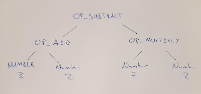
Now if we start at the first sub expression (3+2) we can clearly note from the first open bracket that we must see a close bracket, and that the expression inside that bracket must be valid on its own. Not only that but regardless of the inside we know that the whole expression still has to be valid. Let's focus on this first bracketed expression, let our attention recurse into it so to speak.

This gives us a much easier problem – we just want to get our virtual machine to compute 3 + 2. In this bytecode dialect we would load the two constants, and then add them with OP_ADD like so:

OP_CONSTANT  (00) '3.000000'
OP_CONSTANT  (01) '2.000000'
OP_ADD

The effect of our vm executing these three instructions is that sitting pretty at the top of the stack is the result of the addition. Winning.

Jumping back out from our bracketed expression, our next token is MINUS, at this point we have a fair idea that it must be used in an infix position. In fact whatever token followed the bracketed expression it must be a valid infix operator, if not the expression is over or had a syntax error.

Assuming the best from our user (naive), we handle MINUS the same way we handled the first PLUS. We've already got the first operand on the stack, now we compile the right operand and then write out the bytecode for OP_SUBTRACT.

The right operand is another simple three instructions:

OP_CONSTANT  (02) '7.000000'
OP_CONSTANT  (03) '2.000000'
OP_MULTIPLY

Then we finish our top level binary expression and write a OP_RETURN to return the value at the top of the stack as the execution's result. Our final hand compiled program is:

OP_CONSTANT  (00) '3.000000'
OP_CONSTANT  (01) '2.000000'
OP_ADD
OP_CONSTANT  (02) '7.000000'
OP_CONSTANT  (03) '2.000000'
OP_MULTIPLY
OP_SUBTRACT
OP_RETURN

Ok that wasn't so hard was it? Let's try make our code do that.

We define a parser object which will keep track of where we are, and whether things have all gone horribly wrong:

class Parser(object):
    def __init__(self):
        self.had_error = False
        self.panic_mode = False
        self.current = None
        self.previous = None

The compiler will also be a class, we'll need one of our Scanner instances to pull tokens from, and since the output is a bytecode Chunk let's go ahead and make one of those in our compiler initializer:

class Compiler(object):

    def __init__(self, source):
        self.parser = Parser()
        self.scanner = Scanner(source)
        self.chunk = Chunk()

Since we have this (empty) chunk of bytecode we will make a helper method to add individual bytes. Every instruction will pass from our compiler into an executable program through this simple .

    def emit_byte(self, byte):
        self.current_chunk().write_chunk(byte)

To quote from Bob Nystrom on the Pratt parsing technique:

the implementation is a deceptively-simple handful of deeply intertwined code

I don't actually think I can do justice to this section. Instead I suggest reading his treatment in Pratt Parsers: Expression Parsing Made Easy which explains the magic behind the parsing component. Our only major difference is instead of creating an AST we are going to directly emit bytecode for our VM.

Now that I've absolved myself from taking responsibility in explaining this somewhat tricky concept, I'll discuss some of the code from compiler.py, and walk through what happens for a particular rule.

I'll jump straight to the juicy bit the table of parse rules. We define a ParseRule for each token, and each rule comprises:

  • an optional handler for when the token is as a prefix (e.g. the minus in (-2)),
  • an optional handler for whet the token is used infix (e.g. the slash in 2/47)
  • a precedence value (a number that determines what is of higher precedence)
rules = [
    ParseRule(None,              None,            Precedence.NONE),   # ERROR
    ParseRule(None,              None,            Precedence.NONE),   # EOF
    ParseRule(Compiler.grouping, None,            Precedence.CALL),   # LEFT_PAREN
    ParseRule(None,              None,            Precedence.NONE),   # RIGHT_PAREN
    ParseRule(Compiler.unary,    Compiler.binary, Precedence.TERM),   # MINUS
    ParseRule(None,              Compiler.binary, Precedence.TERM),   # PLUS
    ParseRule(None,              Compiler.binary, Precedence.FACTOR), # SLASH
    ParseRule(None,              Compiler.binary, Precedence.FACTOR), # STAR
    ParseRule(Compiler.number,   None,            Precedence.NONE),   # NUMBER
]

These rules really are the magic of our compiler. When we get to a particular token such as MINUS we see if it is an infix operator and if so we've gone and got its first operand ready. At all times we rely on the relative precedence; consuming everything with higher precedence than the operator we are currently evaluating.

In the expression:

2 + 3 * 4

The * has higher precedence than the +, so 3 * 4 will be parsed together as the second operand to the first infix operator (the +) which follows the BEDMAS order of operations I was taught at high school.

To encode these precedence values we make another Python object moonlighting as an enum:

class Precedence(object):
    NONE = 0
    DEFAULT = 1
    TERM = 2        # + -
    FACTOR = 3      # * /
    UNARY = 4       # ! - +
    CALL = 5        # ()
    PRIMARY = 6

What happens in our compiler when turning -2.0 into bytecode? Assume we've just pulled the token MINUS from the scanner. Every expression has to start with some type of prefix – whether that is:

  • a bracket group (,
  • a number 2,
  • or a prefix unary operator -.

Knowing that, our compiler assumes there is a prefix handler in the rule table – in this case it points us at the unary handler.

    def parse_precedence(self, precedence):
        # parses any expression of a given precedence level or higher
        self.advance()
        prefix_rule = self._get_rule(self.parser.previous.type).prefix
        prefix_rule(self)

unary is called:

    def unary(self):
        op_type = self.parser.previous.type
        # Compile the operand
        self.parse_precedence(Precedence.UNARY)
        # Emit the operator instruction
        if op_type == TokenTypes.MINUS:
            self.emit_byte(OpCode.OP_NEGATE)

Here – before writing the OP_NEGATE opcode we recurse back into parse_precedence to ensure that whatever follows the MINUS token is compiled – provided it has higher precedence than unary – e.g. a bracketed group. Crucially at run time this recursive call will ensure that the result is left on top of our stack. Armed with this knowledge, the unary method just has to emit a single byte with the OP_NEGATE opcode.

Test compilation

Now we can test our compiler by outputting disassembled bytecode of our user entered expressions. Create a new entry_point targetcompiler:

from rpython.rlib import rfile
from compiler import Compiler

LINE_BUFFER_LENGTH = 1024


def entry_point(argv):
    stdin, stdout, stderr = rfile.create_stdio()

    try:
        while True:
            stdout.write("> ")
            source = stdin.readline(LINE_BUFFER_LENGTH)
            compiler = Compiler(source, debugging=True)
            compiler.compile()
    except:
        pass
    return 0

Translate it and test it out:

$ ./compiler1 
> (2/4 + 1/2)
== code ==

0000 OP_CONSTANT  (00) '2.000000'
0002 OP_CONSTANT  (01) '4.000000'
0004 OP_DIVIDE    
0005 OP_CONSTANT  (02) '1.000000'
0007 OP_CONSTANT  (00) '2.000000'
0009 OP_DIVIDE    
0010 OP_ADD       
0011 OP_RETURN

Now if you've made it this far you'll be eager to finally connect everything together by executing this bytecode with the virtual machine.

End to end

All the pieces slot together rather easily at this point, create a new file targetcalc.py and define our entry point:

from rpython.rlib import rfile
from compiler import Compiler
from vm import VM

LINE_BUFFER_LENGTH = 4096


def entry_point(argv):
    stdin, stdout, stderr = rfile.create_stdio()
    vm = VM()
    try:
        while True:
            stdout.write("> ")
            source = stdin.readline(LINE_BUFFER_LENGTH)
            if source:
                compiler = Compiler(source, debugging=False)
                compiler.compile()
                vm.interpret_chunk(compiler.chunk)
    except:
        pass
    return 0


def target(driver, *args):
    driver.exe_name = "calc"
    return entry_point, None

Let's try catch it out with a double negative:

$ ./calc 
> 2--3
== VM TRACE ==
          []
0000 OP_CONSTANT  (00) '2.000000'
          [ 2.000000 ]
0002 OP_CONSTANT  (01) '3.000000'
          [ 2.000000 ] [ 3.000000 ]
0004 OP_NEGATE    
          [ 2.000000 ] [ -3.000000 ]
0005 OP_SUBTRACT  
          [ 5.000000 ]
0006 OP_RETURN    
5.000000

Ok well let's evaluate the first 50 terms of the Nilakantha Series:

$ ./calc
> 3 + 4 * ((1/(2 * 3 * 4)) + (1/(4 * 5 * 6)) - (1/(6 * 7 * 8)) + (1/(8 * 9 * 10)) - (1/(10 * 11 * 12)) + (1/(12 * 13 * 14)) - (1/(14 * 15 * 16)) + (1/(16 * 17 * 18)) - (1/(18 * 19 * 20)) + (1/(20 * 21 * 22)) - (1/(22 * 23 * 24)) + (1/(24 * 25 * 26)) - (1/(26 * 27 * 28)) + (1/(28 * 29 * 30)) - (1/(30 * 31 * 32)) + (1/(32 * 33 * 34)) - (1/(34 * 35 * 36)) + (1/(36 * 37 * 38)) - (1/(38 * 39 * 40)) + (1/(40 * 41 * 42)) - (1/(42 * 43 * 44)) + (1/(44 * 45 * 46)) - (1/(46 * 47 * 48)) + (1/(48 * 49 * 50)) - (1/(50 * 51 * 52)) + (1/(52 * 53 * 54)) - (1/(54 * 55 * 56)) + (1/(56 * 57 * 58)) - (1/(58 * 59 * 60)) + (1/(60 * 61 * 62)) - (1/(62 * 63 * 64)) + (1/(64 * 65 * 66)) - (1/(66 * 67 * 68)) + (1/(68 * 69 * 70)) - (1/(70 * 71 * 72)) + (1/(72 * 73 * 74)) - (1/(74 * 75 * 76)) + (1/(76 * 77 * 78)) - (1/(78 * 79 * 80)) + (1/(80 * 81 * 82)) - (1/(82 * 83 * 84)) + (1/(84 * 85 * 86)) - (1/(86 * 87 * 88)) + (1/(88 * 89 * 90)) - (1/(90 * 91 * 92)) + (1/(92 * 93 * 94)) - (1/(94 * 95 * 96)) + (1/(96 * 97 * 98)) - (1/(98 * 99 * 100)) + (1/(100 * 101 * 102)))

== VM TRACE ==
          []
0000 OP_CONSTANT  (00) '3.000000'
          [ 3.000000 ]
0002 OP_CONSTANT  (01) '4.000000'
...SNIP...
0598 OP_CONSTANT  (101) '102.000000'
          [ 3.000000 ] [ 4.000000 ] [ 0.047935 ] [ 1.000000 ] [ 10100.000000 ] [ 102.000000 ]
0600 OP_MULTIPLY  
          [ 3.000000 ] [ 4.000000 ] [ 0.047935 ] [ 1.000000 ] [ 1030200.000000 ]
0601 OP_DIVIDE    
          [ 3.000000 ] [ 4.000000 ] [ 0.047935 ] [ 0.000001 ]
0602 OP_ADD       
          [ 3.000000 ] [ 4.000000 ] [ 0.047936 ]
0603 OP_MULTIPLY  
          [ 3.000000 ] [ 0.191743 ]
0604 OP_ADD       
          [ 3.191743 ]
0605 OP_RETURN    
3.191743

We just executed 605 virtual machine instructions to compute pi to 1dp!

This brings us to the end of this tutorial. To recap we've walked through the whole compilation process: from the user providing an expression string on the REPL, scanning the source string into tokens, parsing the tokens while accounting for relative precedence via a Pratt parser, generating bytecode, and finally executing the bytecode on our own VM. RPython translated what we wrote into C and compiled it, meaning our resulting calc REPL is really fast.

“The world is a thing of utter inordinate complexity and richness and strangeness that is absolutely awesome.”

― Douglas Adams

Many thanks to Bob Nystrom for writing the book that inspired this post, and thanks to Carl Friedrich and Matt Halverson for reviewing.

― Brian (@thorneynzb)

Friday, September 21, 2018

Inside cpyext: Why emulating CPython C API is so Hard


cpyext is PyPy's subsystem which provides a compatibility layer to compile and run CPython C extensions inside PyPy. Often people ask why a particular C extension doesn't work or is very slow on PyPy. Usually it is hard to answer without going into technical details. The goal of this blog post is to explain some of these technical details, so that we can simply link here instead of explaining again and again :).
From a 10.000 foot view, cpyext is PyPy's version of "Python.h". Every time you compile an extension which uses that header file, you are using cpyext. This includes extension explicitly written in C (such as numpy) and extensions which are generated from other compilers/preprocessors (e.g. Cython).
At the time of writing, the current status is that most C extensions "just work". Generally speaking, you can simply pip install them, provided they use the public, official C API instead of poking at private implementation details. However, the performance of cpyext is generally poor. A Python program which makes heavy use of cpyext extensions is likely to be slower on PyPy than on CPython.
Note: in this blog post we are talking about Python 2.7 because it is still the default version of PyPy: however most of the implementation of cpyext is shared with PyPy3, so everything applies to that as well.

C API Overview

In CPython, which is written in C, Python objects are represented as PyObject*, i.e. (mostly) opaque pointers to some common "base struct".
CPython uses a very simple memory management scheme: when you create an object, you allocate a block of memory of the appropriate size on the heap. Depending on the details, you might end up calling different allocators, but for the sake of simplicity, you can think that this ends up being a call to malloc(). The resulting block of memory is initialized and casted to to PyObject*: this address never changes during the object lifetime, and the C code can freely pass it around, store it inside containers, retrieve it later, etc.
Memory is managed using reference counting. When you create a new reference to an object, or you discard a reference you own, you have to increment or decrement the reference counter accordingly. When the reference counter goes to 0, it means that the object is no longer used and can safely be destroyed. Again, we can simplify and say that this results in a call to free(), which finally releases the memory which was allocated by malloc().
Generally speaking, the only way to operate on a PyObject* is to call the appropriate API functions. For example, to convert a given PyObject* to a C integer, you can use PyInt_AsLong(); to add two objects together, you can call PyNumber_Add().
Internally, PyPy uses a similar approach. All Python objects are subclasses of the RPython W_Root class, and they are operated by calling methods on the space singleton, which represents the interpreter.
At first, it looks very easy to write a compatibility layer: just make PyObject* an alias for W_Root, and write simple RPython functions (which will be translated to C by the RPython compiler) which call the space accordingly:
def PyInt_AsLong(space, o):
    return space.int_w(o)

def PyNumber_Add(space, o1, o2):
    return space.add(o1, o2)
Actually, the code above is not too far from the real implementation. However, there are tons of gory details which make it much harder than it looks, and much slower unless you pay a lot of attention to performance.

The PyPy GC

To understand some of cpyext challenges, you need to have at least a rough idea of how the PyPy GC works.
Contrarily to the popular belief, the "Garbage Collector" is not only about collecting garbage: instead, it is generally responsible for all memory management, including allocation and deallocation.
Whereas CPython uses a combination of malloc/free/refcounting to manage memory, the PyPy GC uses a completely different approach. It is designed assuming that a dynamic language like Python behaves the following way:
  • You create, either directly or indirectly, lots of objects.
  • Most of these objects are temporary and very short-lived. Think e.g. of doing a + b + c: you need to allocate an object to hold the temporary result of a + b, then it dies very quickly because you no longer need it when you do the final + c part.
  • Only small fraction of the objects survive and stay around for a while.
So, the strategy is: make allocation as fast as possible; make deallocation of short-lived objects as fast as possible; find a way to handle the remaining small set of objects which actually survive long enough to be important.
This is done using a Generational GC: the basic idea is the following:
  1. We have a nursery, where we allocate "young objects" very quickly.
  2. When the nursery is full, we start what we call a "minor collection".
    • We do a quick scan to determine the small set of objects which survived so far
    • We move these objects out of the nursery, and we place them in the area of memory which contains the "old objects". Since the address of the objects changes, we fix all the references to them accordingly.
  1. now the nursery contains only objects which "died young". We can discard all of them very quickly, reset the nursery, and use the same area of memory to allocate new objects from now.
In practice, this scheme works very well and it is one of the reasons why PyPy is much faster than CPython. However, careful readers have surely noticed that this is a problem for cpyext. On one hand, we have PyPy objects which can potentially move and change their underlying memory address; on the other hand, we need a way to represent them as fixed-address PyObject* when we pass them to C extensions. We surely need a way to handle that.

PyObject* in PyPy

Another challenge is that sometimes, PyObject* structs are not completely opaque: there are parts of the public API which expose to the user specific fields of some concrete C struct. For example the definition of PyTypeObject which exposes many of the tp_* slots to the user. Since the low-level layout of PyPy W_Root objects is completely different than the one used by CPython, we cannot simply pass RPython objects to C; we need a way to handle the difference.
So, we have two issues so far: objects can move, and incompatible low-level layouts. cpyext solves both by decoupling the RPython and the C representations. We have two "views" of the same entity, depending on whether we are in the PyPy world (the movable W_Root subclass) or in the C world (the non-movable PyObject*).
PyObject* are created lazily, only when they are actually needed. The vast majority of PyPy objects are never passed to any C extension, so we don't pay any penalty in that case. However, the first time we pass a W_Root to C, we allocate and initialize its PyObject* counterpart.
The same idea applies also to objects which are created in C, e.g. by calling PyObject_New(). At first, only the PyObject* exists and it is exclusively managed by reference counting. As soon as we pass it to the PyPy world (e.g. as a return value of a function call), we create its W_Root counterpart, which is managed by the GC as usual.
Here we start to see why calling cpyext modules is more costly in PyPy than in CPython. We need to pay some penalty for all the conversions between W_Root and PyObject*.
Moreover, the first time we pass a W_Root to C we also need to allocate the memory for the PyObject* using a slowish "CPython-style" memory allocator. In practice, for all the objects which are passed to C we pay more or less the same costs as CPython, thus effectively "undoing" the speedup guaranteed by PyPy's Generational GC under normal circumstances.

Crossing the border between RPython and C

There are two other things we need to care about whenever we cross the border between RPython and C, and vice-versa: exception handling and the GIL.
In the C API, exceptions are raised by calling PyErr_SetString() (or one of many other functions which have a similar effect), which basically works by creating an exception value and storing it in some global variable. The function then signals that an exception has occurred by returning an error value, usually NULL.
On the other hand, in the PyPy interpreter, exceptions are propagated by raising the RPython-level OperationError exception, which wraps the actual app-level exception values. To harmonize the two worlds, whenever we return from C to RPython, we need to check whether a C API exception was raised and if so turn it into an OperationError.
We won't dig into details of how the GIL is handled in cpyext. For the purpose of this post, it is enough to know that whenever we enter C land, we store the current thread id into a global variable which is accessible also from C; conversely, whenever we go back from RPython to C, we restore this value to 0.
Similarly, we need to do the inverse operations whenever you need to cross the border between C and RPython, e.g. by calling a Python callback from C code.
All this complexity is automatically handled by the RPython function generic_cpy_call. If you look at the code you see that it takes care of 4 things:
  1. Handling the GIL as explained above.
  2. Handling exceptions, if they are raised.
  3. Converting arguments from W_Root to PyObject*.
  4. Converting the return value from PyObject* to W_Root.
So, we can see that calling C from RPython introduce some overhead. Can we measure it?
Assuming that the conversion between W_Root and PyObject* has a reasonable cost (as explained by the previous section), the overhead introduced by a single border-cross is still acceptable, especially if the callee is doing some non-negligible amount of work.
However this is not always the case. There are basically three problems that make (or used to make) cpyext super slow:
  1. Paying the border-crossing cost for trivial operations which are called very often, such as Py_INCREF.
  2. Crossing the border back and forth many times, even if it's not strictly needed.
  3. Paying an excessive cost for argument and return value conversions.
The next sections explain in more detail each of these problems.

Avoiding unnecessary roundtrips

Prior to the 2017 Cape Town Sprint, cpyext was horribly slow, and we were well aware of it: the main reason was that we never really paid too much attention to performance. As explained in the blog post, emulating all the CPython quirks is basically a nightmare, so better to concentrate on correctness first.
However, we didn't really know why it was so slow. We had theories and assumptions, usually pointing at the cost of conversions between W_Root and PyObject*, but we never actually measured it.
So, we decided to write a set of cpyext microbenchmarks to measure the performance of various operations. The result was somewhat surprising: the theory suggests that when you do a cpyext C call, you should pay the border-crossing costs only once, but what the profiler told us was that we were paying the cost of generic_cpy_call several times more than what we expected.
After a bit of investigation, we discovered this was ultimately caused by our "correctness-first" approach. For simplicity of development and testing, when we started cpyext we wrote everything in RPython: thus, every single API call made from C (like the omnipresent PyArg_ParseTuple(), PyInt_AsLong(), etc.) had to cross back the C-to-RPython border. This was especially daunting for very simple and frequent operations like Py_INCREF and Py_DECREF, which CPython implements as a single assembly instruction!
Another source of slow down was the implementation of PyTypeObject slots. At the C level, these are function pointers which the interpreter calls to do certain operations, e.g. tp_new to allocate a new instance of that type.
As usual, we have some magic to implement slots in RPython; in particular, _make_wrapper does the opposite of generic_cpy_call: it takes a RPython function and wraps it into a C function which can be safely called from C, handling the GIL, exceptions and argument conversions automatically.
This was very handy during the development of cpyext, but it might result in some bad nonsense; consider what happens when you call the following C function:
static PyObject* foo(PyObject* self, PyObject* args)
{
    PyObject* result = PyInt_FromLong(1234);
    return result;
}
  1. you are in RPython and do a cpyext call to foo: RPython-to-C;
  2. foo calls PyInt_FromLong(1234), which is implemented in RPython: C-to-RPython;
  3. the implementation of PyInt_FromLong indirectly calls PyIntType.tp_new, which is a C function pointer: RPython-to-C;
  4. however, tp_new is just a wrapper around an RPython function, created by _make_wrapper: C-to-RPython;
  5. finally, we create our RPython W_IntObject(1234); at some point during the RPython-to-C crossing, its PyObject* equivalent is created;
  6. after many layers of wrappers, we are again in foo: after we do return result, during the C-to-RPython step we convert it from PyObject* to W_IntObject(1234).
Phew! After we realized this, it was not so surprising that cpyext was very slow :). And this was a simplified example, since we are not passing a PyObject* to the API call. When we do, we need to convert it back and forth at every step. Actually, I am not even sure that what I described was the exact sequence of steps which used to happen, but you get the general idea.
The solution is simple: rewrite as much as we can in C instead of RPython, to avoid unnecessary roundtrips. This was the topic of most of the Cape Town sprint and resulted in the cpyext-avoid-roundtrip branch, which was eventually merged.
Of course, it is not possible to move everything to C: there are still operations which need to be implemented in RPython. For example, think of PyList_Append: the logic to append an item to a list is complex and involves list strategies, so we cannot replicate it in C. However, we discovered that a large subset of the C API can benefit from this.
Moreover, the C API is huge. While we invented this new way of writing cpyext code, we still need to convert many of the functions to the new paradigm. Sometimes the rewrite is not automatic or straighforward. cpyext is a delicate piece of software, so it happens often that we make a mistake and end up staring at a segfault in gdb.
However, the most important takeaway is that the performance improvements we got from this optimization are impressive, as we will detail later.

Conversion costs

The other potential big source of slowdown is the conversion of arguments between W_Root and PyObject*.
As explained earlier, the first time you pass a W_Root to C, you need to allocate its PyObject* counterpart. Suppose you have a foo function defined in C, which takes a single int argument:
for i in range(N):
    foo(i)
To run this code, you need to create a different PyObject* for each value of i: if implemented naively, it means calling N times malloc() and free(), which kills performance.
CPython has the very same problem, which is solved by using a free list to allocate ints. So, what we did was to simply steal the code from CPython and do the exact same thing. This was also done in the cpyext-avoid-roundtrip branch, and the benchmarks show that it worked perfectly.
Every type which is converted often to PyObject* must have a very fast allocator. At the moment of writing, PyPy uses free lists only for ints and tuples: one of the next steps on our TODO list is certainly to use this technique with more types, like float.
Conversely, we also need to optimize the converstion from PyObject* to W_Root: this happens when an object is originally allocated in C and returned to Python. Consider for example the following code:
import numpy as np
myarray = np.random.random(N)
for i in range(len(arr)):
    myarray[i]
At every iteration, we get an item out of the array: the return type is a an instance of numpy.float64 (a numpy scalar), i.e. a PyObject'*: this is something which is implemented by numpy entirely in C, so completely opaque to cpyext. We don't have any control on how it is allocated, managed, etc., and we can assume that allocation costs are the same as on CPython.
As soon as we return these PyObject* to Python, we need to allocate their W_Root equivalent. If you do it in a small loop like in the example above, you end up allocating all these W_Root inside the nursery, which is a good thing since allocation is super fast (see the section above about the PyPy GC).
However, we also need to keep track of the W_Root to PyObject* link. Currently, we do this by putting all of them in a dictionary, but it is very inefficient, especially because most of these objects die young and thus it is wasted work to do that for them. Currently, this is one of the biggest unresolved problem in cpyext, and it is what causes the two microbenchmarks allocate_int and allocate_tuple to be very slow.
We are well aware of the problem, and we have a plan for how to fix it. The explanation is too technical for the scope of this blog post as it requires a deep knowledge of the GC internals to be understood, but the details are here.

C API quirks

Finally, there is another source of slowdown which is beyond our control. Some parts of the CPython C API are badly designed and expose some of the implementation details of CPython.
The major example is reference counting. The Py_INCREF / Py_DECREF API is designed in such a way which forces other implementation to emulate refcounting even in presence of other GC management schemes, as explained above.
Another example is borrowed references. There are API functions which do not incref an object before returning it, e.g. PyList_GetItem(). This is done for performance reasons because we can avoid a whole incref/decref pair, if the caller needs to handle the returned item only temporarily: the item is kept alive because it is in the list anyway.
For PyPy, this is a challenge: thanks to list strategies, lists are often represented in a compact way. For example, a list containing only integers is stored as a C array of long. How to implement PyList_GetItem? We cannot simply create a PyObject* on the fly, because the caller will never decref it and it will result in a memory leak.
The current solution is very inefficient. The first time we do a PyList_GetItem, we convert the whole list to a list of PyObject*. This is bad in two ways: the first is that we potentially pay a lot of unneeded conversion cost in case we will never access the other items of the list. The second is that by doing that we lose all the performance benefit granted by the original list strategy, making it slower for the rest of the pure-python code which will manipulate the list later.
PyList_GetItem is an example of a bad API because it assumes that the list is implemented as an array of PyObject*: after all, in order to return a borrowed reference, we need a reference to borrow, don't we?
Fortunately, (some) CPython developers are aware of these problems, and there is an ongoing project to design a better C API which aims to fix exactly this kind of problem.
Nonetheless, in the meantime we still need to implement the current half-broken APIs. There is no easy solution for that, and it is likely that we will always need to pay some performance penalty in order to implement them correctly.
However, what we could potentially do is to provide alternative functions which do the same job but are more PyPy friendly: for example, we could think of implementing PyList_GetItemNonBorrowed or something like that: then, C extensions could choose to use it (possibly hidden inside some macro and #ifdef) if they want to be fast on PyPy.

Current performance

During the whole blog post we claimed cpyext is slow. How slow it is, exactly?
We decided to concentrate on microbenchmarks for now. It should be evident by now there are simply too many issues which can slow down a cpyext program, and microbenchmarks help us to concentrate on one (or few) at a time.
The microbenchmarks measure very simple things, like calling functions and methods with the various calling conventions (no arguments, one arguments, multiple arguments); passing various types as arguments (to measure conversion costs); allocating objects from C, and so on.
Here are the results from the old PyPy 5.8 relative and normalized to CPython 2.7, the lower the better:


PyPy was horribly slow everywhere, ranging from 2.5x to 10x slower. It is particularly interesting to compare simple.noargs, which measures the cost of calling an empty function with no arguments, and simple.onearg(i), which measures the cost calling an empty function passing an integer argument: the latter is ~2x slower than the former, indicating that the conversion cost of integers is huge.
PyPy 5.8 was the last release before the famous Cape Town sprint, when we started to look at cpyext performance seriously. Here are the performance data for PyPy 6.0, the latest release at the time of writing:


The results are amazing! PyPy is now massively faster than before, and for most benchmarks it is even faster than CPython: yes, you read it correctly: PyPy is faster than CPython at doing CPython's job, even considering all the extra work it has to do to emulate the C API. This happens thanks to the JIT, which produces speedups high enough to counterbalance the slowdown caused by cpyext.
There are two microbenchmarks which are still slower though: allocate_int and allocate_tuple, for the reasons explained in the section about Conversion costs.

Next steps

Despite the spectacular results we got so far, cpyext is still slow enough to kill performance in most real-world code which uses C extensions extensively (e.g., the omnipresent numpy).
Our current approach is something along these lines:
  1. run a real-world small benchmark which exercises cpyext
  2. measure and find the major bottleneck
  3. write a corresponding microbenchmark
  4. optimize it
  5. repeat
On one hand, this is a daunting task because the C API is huge and we need to tackle functions one by one. On the other hand, not all the functions are equally important, and is is enough to optimize a relatively small subset to improve many different use cases.
Where a year ago we announced we have a working answer to run c-extension in PyPy, we now have a clear picture of what are the performance bottlenecks, and we have developed some technical solutions to fix them. It is "only" a matter of tackling them, one by one. It is worth noting that most of the work was done during two sprints, for a total 2-3 person-months of work.
We think this work is important for the Python ecosystem. PyPy has established a baseline for performance in pure python code, providing an answer for the "Python is slow" detractors. The techniques used to make cpyext performant will let PyPy become an alternative for people who mix C extensions with Python, which, it turns out, is just about everyone, in particular those using the various scientific libraries. Today, many developers are forced to seek performance by converting code from Python to a lower language. We feel there is no reason to do this, but in order to prove it we must be able to run both their python and their C extensions performantly, then we can begin to educate them how to write JIT-friendly code in the first place.
We envision a future in which you can run arbitrary Python programs on PyPy, with the JIT speeding up the pure Python parts and the C parts running as fast as today: the best of both worlds!

Sunday, September 9, 2018

The First 15 Years of PyPy — a Personal Retrospective

A few weeks ago I (=Carl Friedrich Bolz-Tereick) gave a keynote at ICOOOLPS in Amsterdam with the above title. I was very happy to have been given that opportunity, since a number of our papers have been published at ICOOOLPS, including the very first one I published when I'd just started my PhD. I decided to turn the talk manuscript into a (longish) blog post, to make it available to a wider audience. Note that this blog post describes my personal recollections and research, it is thus necessarily incomplete and coloured by my own experiences.

PyPy has turned 15 years old this year, so I decided that that's a good reason to dig into and talk about the history of the project so far. I'm going to do that using the lens of how performance developed over time, which is from something like 2000x slower than CPython, to roughly 7x faster. In this post I am going to present the history of the project, and also talk about some lessons that we learned.

The post does not make too many assumptions about any prior knowledge of what PyPy is, so if this is your first interaction with it, welcome! I have tried to sprinkle links to earlier blog posts and papers into the writing, in case you want to dive deeper into some of the topics.

As a disclaimer, in this post I am going to mostly focus on ideas, and not explain who had or implemented them. A huge amount of people contributed to the design, the implementation, the funding and the organization of PyPy over the years, and it would be impossible to do them all justice.

2003: Starting the Project

On the technical level PyPy is a Python interpreter written in Python, which is where the name comes from. It also has an automatically generated JIT compiler, but I'm going to introduce that gradually over the rest of the blog post, so let's not worry about it too much yet. On the social level PyPy is an interesting mixture of a open source project, that sometimes had research done in it.

The project got started in late 2002 and early 2003. To set the stage, at that point Python was a significantly less popular language than it is today. Python 2.2 was the version at the time, Python didn't even have a bool type yet.

In fall 2002 the PyPy project was started by a number of Python programmers on a mailing list who said something like (I am exaggerating somewhat) "Python is the greatest most wonderful most perfect language ever, we should use it for absolutely everything. Well, what aren't we using it for? The Python virtual machine itself is written in C, that's bad. Let's start a project to fix that."

Originally that project was called "minimal python", or "ptn", later gradually renamed to PyPy. Here's the mailing list post to announce the project more formally:

Minimal Python Discussion, Coding and Sprint
--------------------------------------------

We announce a mailinglist dedicated to developing
a "Minimal Python" version.  Minimal means that
we want to have a very small C-core and as much
as possible (re)implemented in python itself.  This
includes (parts of) the VM-Code.

Why would that kind of project be useful? Originally it wasn't necessarily meant to be useful as a real implementation at all, it was more meant as a kind of executable explanation of how Python works, free of the low level details of CPython. But pretty soon there were then also plans for how the virtual machine (VM) could be bootstrapped to be runnable without an existing Python implementation, but I'll get to that further down.

2003: Implementing the Interpreter

In early 2003 a group of Python people met in Hildesheim (Germany) for the first of many week long development sprints, organized by Holger Krekel. During that week a group of people showed up and started working on the core interpreter. In May 2003 a second sprint was organized by Laura Creighton and Jacob Halén in Gothenburg (Sweden). And already at that sprint enough of the Python bytecodes and data structures were implemented to make it possible to run a program that computed how much money everybody had to pay for the food bills of the week. And everybody who's tried that for a large group of people knows that that’s an amazingly complex mathematical problem.

In the next two years, the project continued as a open source project with various contributors working on it in their free time, and meeting for the occasional sprint. In that time, the rest of the core interpreter and the core data types were implemented.

There's not going to be any other code in this post, but to give a bit of a flavor of what the Python interpreter at that time looked like, here's the implementation of the DUP_TOP bytecode after these first sprints. As you can see, it's in Python, obviously, and it has high level constructs such as method calls to do the stack manipulations:

def DUP_TOP(f):
    w_1 = f.valuestack.top()
    f.valuestack.push(w_1)

Here's the early code for integer addition:

def int_int_add(space, w_int1, w_int2):
    x = w_int1.intval
    y = w_int2.intval
    try:
        z = x + y
    except OverflowError:
        raise FailedToImplement(space.w_OverflowError,
                                space.wrap("integer addition"))
    return W_IntObject(space, z)

(the current implementations look slightly but not fundamentally different.)

Early organizational ideas

Some of the early organizational ideas of the project were as follows. Since the project was started on a sprint and people really liked that style of working PyPy continued to be developed on various subsequent sprints.

From early on there was a very heavy emphasis on testing. All the parts of the interpreter that were implemented had a very careful set of unit tests to make sure that they worked correctly. From early on, there was a continuous integration infrastructure, which grew over time (nowadays it is very natural for people to have automated tests, and the concept of green/red builds: but embracing this workflow in the early 2000s was not really mainstream yet, and it is probably one of the reasons behind PyPy's success).

At the sprints there was also an emphasis on doing pair programming to make sure that everybody understood the codebase equally. There was also a heavy emphasis on writing good code and on regularly doing refactorings to make sure that the codebase remained nice, clean and understandable. Those ideas followed from the early thoughts that PyPy would be a sort of readable explanation of the language.

There was also a pretty fundamental design decision made at the time. That was that the project should stay out of language design completely. Instead it would follow CPython's lead and behave exactly like that implementation in all cases. The project therefore committed to being almost quirk-to-quirk compatible and to implement even the more obscure (and partially unnecessary) corner cases of CPython.

All of these principles continue pretty much still today (There are a few places where we had to deviate from being completely compatible, they are documented here).

2004-2007: EU-Funding

While all this coding was going on it became clear pretty soon that the goals that various participants had for the project would be very hard to achieve with just open source volunteers working on the project in their spare time. Particularly also the sprints became expensive given that those were just volunteers doing this as a kind of weird hobby. Therefore a couple of people of the project got together to apply for an EU grant in the framework programme 6 to solve these money problems. In mid-2004 that application proved to be successful. And so the project got a grant of a 1.3 million Euro for two years to be able to employ some of the core developers and to make it possible for them work on the project full time. The EU grant went to seven small-to-medium companies and Uni Düsseldorf. The budget also contained money to fund sprints, both for the employed core devs as well as other open source contributors.

The EU project started in December 2004 and that was a fairly heavy change in pace for the project. Suddenly a lot of people were working full time on it, and the pace and the pressure picked up quite a lot. Originally it had been a leisurely project people worked on for fun. But afterwards people discovered that doing this kind of work full time becomes slightly less fun, particularly also if you have to fulfill the ambitious technical goals that the EU proposal contained. And the proposal indeed contained a bit everything to increase its chance of acceptance, such as aspect oriented programming, semantic web, logic programming, constraint programming, and so on. Unfortunately it turned out that those things then have to be implemented, which can be called the first thing we learned: if you promise something to the EU, you'll have to actually go do it (After the funding ended, a lot of these features were actually removed from the project again, at a cleanup sprint).

2005: Bootstrapping PyPy

So what were the actually useful things done as part of the EU project?

One of the most important goals that the EU project was meant to solve was the question of how to turn PyPy into an actually useful VM for Python. The bootstrapping plans were taken quite directly from Squeak, which is a Smalltalk VM written in a subset of Smalltalk called Slang, which can then be bootstrapped to C code. The plan for PyPy was to do something similar, to define a restricted subset of Python called RPython, restricted in such a way that it should be possible to statically compile RPython programs to C code. Then the Python interpreter should only use that subset, of course.

The main difference from the Squeak approach is that Slang, the subset of Squeak used there, is actually quite a low level language. In a way, you could almost describe it as C with Smalltalk syntax. RPython was really meant to be a much higher level language, much closer to Python, with full support for single inheritance classes, and most of Python's built-in data structures.

(BTW, you don’t have to understand any of the illustrations in this blog post, they are taken from talks and project reports we did over the years so they are of archaeological interest only and I don’t understand most of them myself.)

From 2005 on, work on the RPython type inference engine and C backend started in earnest, which was sort of co-developed with the RPython language definition and the PyPy Python interpreter. This is also roughly the time that I joined the project as a volunteer.

And at the second sprint I went to, in July 2005, two and a half years after the project got started, we managed to bootstrap the PyPy interpreter to C for the first time. When we ran the compiled program, it of course immediately segfaulted. The reason for that was that the C backend had turned characters into signed chars in C, while the rest of the infrastructure assumed that they were unsigned chars. After we fixed that, the second attempt worked and we managed to run an incredibly complex program, something like 6 * 7. That first bootstrapped version was really really slow, a couple of hundred times slower than CPython.

The bootstrapping process of RPython has a number of nice benefits, a big one being that a number of the properties of the generated virtual machine don't have to expressed in the interpreter. The biggest example of this is garbage collection. RPython is a garbage collected language, and the interpreter does not have to care much about GC in most cases. When the C source code is generated, a GC is automatically inserted. This is a source of great flexibility. Over time we experimented with a number of different GC approaches, from reference counting to Boehm to our current incremental generational collector. As an aside, for a long time we were also working on other backends to the RPython language and hoped to be able to target Java and .NET as well. Eventually we abandoned this strand of work, however.

RPython's Modularity Problems

Now we come to the first thing I would say we learned in the project, which is that the quality of tools we thought of as internal things still matters a lot. One of the biggest technical mistakes we've made in the project was that we designed RPython without any kind of story for modularity. There is no concept of modules in the language or any other way to break up programs into smaller components. We always thought that it would be ok for RPython to be a little bit crappy. It was meant to be this sort of internal language with not too many external users. And of course that turned out to be completely wrong later.

That lack of modularity led to various problems that persist until today. The biggest one is that there is no separate compilation for RPython programs at all! You always need to compile all the parts of your VM together, which leads to infamously bad compilation times.

Also by not considering the modularity question we were never forced to fix some internal structuring issues of the RPython compiler itself. Various layers of the compiler keep very badly defined and porous interfaces between them. This was made possible by being able to work with all the program information in one heap, making the compiler less approachable and maintainable than it maybe could be.

Of course this mistake just got more and more costly to fix over time, and so it means that so far nobody has actually done it. Not thinking more carefully about RPython's design, particularly its modularity story, is in my opinion the biggest technical mistake the project made.

2006: The Meta-JIT

After successfully bootstrapping the VM we did some fairly straightforward optimizations on the interpreter and the C backend and managed to reduce the slowdown versus CPython to something like 2-5 times slower. That's great! But of course not actually useful in practice. So where do we go from here?

One of the not so secret goals of Armin Rigo, one of the PyPy founders, was to use PyPy together with some advanced partial evaluation magic sauce to somehow automatically generate a JIT compiler from the interpreter. The goal was something like, "you write your interpreter in RPython, add a few annotations and then we give you a JIT for free for the language that that interpreter implements."

Where did the wish for that approach come from, why not just write a JIT for Python manually in the first place? Armin had actually done just that before he co-founded PyPy, in a project called Psyco. Psyco was an extension module for CPython that contained a method-based JIT compiler for Python code. And Psyco proved to be an amazingly frustrating compiler to write. There were two main reasons for that. The first reason was that Python is actually quite a complex language underneath its apparent simplicity. The second reason for the frustration was that Python was and is very much an alive language, that gains new features in the language core in every version. So every time a new Python version came out, Armin had to do fundamental changes and rewrites to Psyco, and he was getting pretty frustrated with it. So he hoped that that effort could be diminished by not writing the JIT for PyPy by hand at all. Instead, the goal was to generate a method-based JIT from the interpreter automatically. By taking the interpreter, and applying a kind of advanced transformation to it, that would turn it into a method-based JIT. And all that would still be translated into a C-based VM, of course.

Slide from Psyco presentation at EuroPython 2002

The First JIT Generator

From early 2006 on until the end of the EU project a lot of work went into writing such a JIT generator. The idea was to base it on runtime partial evaluation. Partial evaluation is an old idea in computer science. It's supposed to be a way to automatically turn interpreters for a language into a compiler for that same language. Since PyPy was trying to generate a JIT compiler, which is in any case necessary to get good performance for a dynamic language like Python, the partial evaluation was going to happen at runtime.

There are various ways to look at partial evaluation, but if you've never heard of it before, a simple way to view it is that it will compile a Python function by gluing together the implementations of the bytecodes of that function and optimizing the result.

The main new ideas of PyPy's partial-evaluation based JIT generator as opposed to earlier partial-evaluation approaches are the ideas of "promote" and the idea of "virtuals". Both of these techniques had already been present (in a slightly less general form) in Psyco, and the goal was to keep using them in PyPy. Both of these techniques also still remain in use today in PyPy. I'm going on a slight technical diversion now, to give a high level explanation of what those ideas are for.

Promote

One important ingredient of any JIT compiler is the ability to do runtime feedback. Runtime feedback is most commonly used to know something about which concrete types are used by a program in practice. Promote is basically a way to easily introduce runtime feedback into the JIT produced by the JIT generator. It's an annotation the implementer of a language can use to express their wish that specialization should happen at this point. This mechanism can be used to express all kinds of runtime feedback, moving values from the interpreter into the compiler, whether they be types or other things.

Virtuals

Virtuals are a very aggressive form of partial escape analysis. A dynamic language often puts a lot of pressure on the garbage collector, since most primitive types (like integers, floats and strings) are boxed in the heap, and new boxes are allocated all the time.

With the help of virtuals a very significant portion of all allocations in the generated machine code can be completely removed. Even if they can't be removed, often the allocation can be delayed or moved into an error path, or even into a deoptimization path, and thus disappear from the generated machine code completely.

This optimization really is the super-power of PyPy's optimizer, since it doesn't work only for primitive boxes but for any kind of object allocated on the heap with a predictable lifetime.

As an aside, while this kind of partial escape analysis is sort of new for object-oriented languages, it has actually existed in Prolog-based partial evaluation systems since the 80s, because it's just extremely natural there.

JIT Status 2007

So, back to our history. We're now in 2007, at the end of the EU project (you can find the EU-reports we wrote during the projects here). The EU project successfully finished, we survived the final review with the EU. So, what's the 2007 status of the JIT generator? It works kind of, it can be applied to PyPy. It produces a VM with a JIT that will turn Python code into machine code at runtime and run it. However, that machine code is not particularly fast. Also, it tends to generate many megabytes of machine code even for small Python programs. While it's always faster than PyPy without JIT, it's only sometimes faster than CPython, and most of the time Psyco still beats it. On the one hand, this is still an amazing achievement! It's arguably the biggest application of partial evaluation at this point in time! On the other hand, it was still quite disappointing in practice, particularly since some of us had believed at the time that it should have been possible to reach and then surpass the speed of Psyco with this approach.

2007: RSqueak and other languages

After the EU project ended we did all kinds of things. Like sleep for a month for example, and have the cleanup sprint that I already mentioned. We also had a slightly unusual sprint in Bern, with members of the Software Composition Group of Oscar Nierstrasz. As I wrote above, PyPy had been heavily influenced by Squeak Smalltalk, and that group is a heavy user of Squeak, so we wanted to see how to collaborate with them. At the beginning of the sprint, we decided together that the goal of that week should be to try to write a Squeak virtual machine in RPython, and at the end of the week we'd gotten surprisingly far with that goal. Basically most of the bytecodes and the Smalltalk object system worked, we had written an image loader and could run some benchmarks (during the sprint we also regularly updated a blog, the success of which led us to start the PyPy blog).

The development of the Squeak interpreter was very interesting for the project, because it was the first real step that moved RPython from being an implementation detail of PyPy to be a more interesting project in its own right. Basically a language to write interpreters in, with the eventual promise to get a JIT for that language almost for free. That Squeak implementation is now called RSqueak ("Research Squeak").

I'll not go into more details about any of the other language implementations in RPython in this post, but over the years we've had a large variety of language of them done by various people and groups, most of them as research vehicles, but also some as real language implementations. Some very cool research results came out of these efforts, here's a slightly outdated list of some of them.

The use of RPython for other languages complicated the PyPy narrative a lot, and in a way we never managed to recover the simplicity of the original project description "PyPy is Python in Python". Because now it's something like "we have this somewhat strange language, a subset of Python, that's called RPython, and it's good to write interpreters in. And if you do that, we'll give you a JIT for almost free. And also, we used that language to write a Python implementation, called PyPy.". It just doesn't roll off the tongue as nicely.

2008-2009: Four More JIT Generators

Back to the JIT. After writing the first JIT generator as part of the EU project, with somewhat mixed results, we actually wrote several more JIT generator prototypes with different architectures to try to solve some of the problems of the first approach. To give an impression of these prototypes, here’s a list of them.

  • The second JIT generator we started working on in 2008 behaved exactly like the first one, but had a meta-interpreter based architecture, to make it more flexible and easier to experiment with. The meta-interpreter was called the "rainbow interpreter", and in general the JIT is an area where we went somewhat overboard with borderline silly terminology, with notable occurrences of "timeshifter", "blackhole interpreter" etc.

  • The third JIT generator was an experiment based on the second one which changed compilation strategy. While the previous two had compiled many control flow paths of the currently compiled function eagerly, that third JIT was sort of maximally lazy and stopped compilation at every control flow split to avoid guessing which path would actually be useful later when executing the code. This was an attempt to reduce the problem of the first JIT generating way too much machine code. Only later, when execution went down one of the not yet compiled paths would it continue compiling more code. This gives an effect similar to that of lazy basic block versioning.

  • The fourth JIT generator was a pretty strange prototype, a runtime partial evaluator for Prolog, to experiment with various specialization trade-offs. It had an approach that we gave a not at all humble name, called "perfect specialization".

  • The fifth JIT generator is the one that we are still using today. Instead of generating a method-based JIT compiler from our interpreter we switched to generating a tracing JIT compiler. Tracing JIT compilers were sort of the latest fashion at the time, at least for a little while.

2009: Meta-Tracing

So, how did that tracing JIT generator work? A tracing JIT generates code by observing and logging the execution of the running program. This yields a straight-line trace of operations, which are then optimized and compiled into machine code. Of course most tracing systems mostly focus on tracing loops.

As we discovered, it's actually quite simple to apply a tracing JIT to a generic interpreter, by not tracing the execution of the user program directly, but by instead tracing the execution of the interpreter while it is running the user program (here's the paper we wrote about this approach).

So that's what we implemented. Of course we kept the two successful parts of the first JIT, promote and virtuals (both links go to the papers about these features in the meta-tracing context).

Why did we Abandon Partial Evaluation?

So one question I get sometimes asked when telling this story is, why did we think that tracing would work better than partial evaluation (PE)? One of the hardest parts of compilers in general and partial evaluation based systems in particular is the decision when and how much to inline, how much to specialize, as well as the decision when to split control flow paths. In the PE based JIT generator we never managed to control that question. Either the JIT would inline too much, leading to useless compilation of all kinds of unlikely error cases. Or it wouldn't inline enough, preventing necessary optimizations.

Meta tracing solves this problem with a hammer, it doesn't make particularly complex inlining decisions at all. It instead decides what to inline by precisely following what a real execution through the program is doing. Its inlining decisions are therefore very understandable and predictable, and it basically only has one heuristic based on whether the called function contains a loop or not: If the called function contains a loop, we'll never inline it, if it doesn't we always try to inline it. That predictability is actually what was the most helpful, since it makes it possible for interpreter authors to understand why the JIT did what it did and to actually influence its inlining decisions by changing the annotations in the interpreter source. It turns out that simple is better than complex.

2009-2011: The PyJIT Eurostars Project

While we were writing all these JIT prototypes, PyPy had sort of reverted back to being a volunteer-driven open source project (although some of us, like Antonio Cuni and I, had started working for universities and other project members had other sources of funding). But again, while we did the work it became clear that to get an actually working fast PyPy with generated JIT we would need actual funding again for the project. So we applied to the EU again, this time for a much smaller project with less money, in the Eurostars framework. We got a grant for three participants, merlinux, OpenEnd and Uni Düsseldorf, on the order of a bit more than half a million euro. That money was specifically for JIT development and JIT testing infrastructure.

Tracing JIT improvements

When writing the grant we had sat together at a sprint and discussed extensively and decided that we would not switch JIT generation approaches any more. We all liked the tracing approach well enough and thought it was promising. So instead we agreed to try in earnest to make the tracing JIT really practical. So in the Eurostars project we started with implementing sort of fairly standard JIT compiler optimizations for the meta-tracing JIT, such as:

  • constant folding

  • dead code elimination

  • loop invariant code motion (using LuaJIT's approach)

  • better heap optimizations

  • faster deoptimization (which is actually a bit of a mess in the meta-approach)

  • and dealing more efficiently with Python frames objects and the features of Python's debugging facilities

2010: speed.pypy.org

In 2010, to make sure that we wouldn't accidentally introduce speed regressions while working on the JIT, we implemented infrastructure to build PyPy and run our benchmarks nightly. Then, the http://speed.pypy.org website was implemented by Miquel Torres, a volunteer. The website shows the changes in benchmark performance compared to the previous n days. It didn't sound too important at first, but this was (and is) a fantastic tool, and an amazing motivator over the next years, to keep continually improving performance.

Continuous Integration

This actually leads me to something else that I'd say we learned, which is that continuous integration is really awesome, and completely transformative to have for a project. This is not a particularly surprising insight nowadays in the open source community, it's easy to set up continuous integration on Github using Travis or some other CI service. But I still see a lot of research projects that don't have tests, that don't use CI, so I wanted to mention it anyway. As I mentioned earlier in the post, PyPy has a quite serious testing culture, with unit tests written for new code, regression tests for all bugs, and integration tests using the CPython test suite. Those tests are run nightly on a number of architectures and operating systems.

Having all this kind of careful testing is of course necessary, since PyPy is really trying to be a Python implementation that people actually use, not just write papers about. But having all this infrastructure also had other benefits, for example it allows us to trust newcomers to the project very quickly. Basically after your first patch gets accepted, you immediately get commit rights to the PyPy repository. If you screw up, the tests (or the code reviews) are probably going to catch it, and that reduction to the barrier to contributing is just super great.

This concludes my advertisement for testing in this post.

2010: Implementing Python Objects with Maps

So, what else did we do in the Eurostars project, apart from adding traditional compiler optimizations to the tracing JIT and setting up CI infrastructure? Another strand of work, that went on sort of concurrently to the JIT generator improvements, were deep rewrites in the Python runtime, and the Python data structures. I am going to write about two exemplary ones here, maps and storage strategies.

The first such rewrite is fairly standard. Python instances are similar to Javascript objects, in that you can add arbitrary attributes to them at runtime. Originally Python instances were backed by a dictionary in PyPy, but of course in practice most instances of the same class have the same set of attribute names. Therefore we went and implemented Self style maps, which are often called hidden classes in the JS world to represent instances instead. This has two big benefits, it allows you to generate much better machine code for instance attribute access and makes instances use a lot less memory.

2011: Container Storage Strategies

Another important change in the PyPy runtime was rewriting the Python container data structures, such as lists, dictionaries and sets. A fairly straightforward observation about how those are used is that in a significant percentage of cases they contain type-homogeneous data. As an example it's quite common to have lists of only integers, or lists of only strings. So we changed the list, dict and set implementations to use something we called storage strategies. With storage strategies these data structures use a more efficient representations if they contain only primitives of the same type, such as ints, floats, strings. This makes it possible to store the values without boxing them in the underlying data structure. Therefore read and write access are much faster for such type homogeneous containers. Of course when later another data type gets added to such a list, the existing elements need to all be boxed at that point, which is expensive. But we did a study and found out that that happens quite rarely in practice. A lot of that work was done by Lukas Diekmann.

Deep Changes in the Runtime are Necessary

These two are just two examples for a number of fairly fundamental changes in the PyPy runtime and PyPy data structures, probably the two most important ones, but we did many others. That leads me to another thing we learned. If you want to generate good code for a complex dynamic language such as Python, it's actually not enough at all to have a good code generator and good compiler optimizations. That's not going to help you, if your runtime data-structures aren't in a shape where it's possible to generate efficient machine code to access them.

Maybe this is well known in the VM and research community. However it's the main mistake that in my opinion every other Python JIT effort has made in the last 10 years, where most projects said something along the lines of "we're not changing the existing CPython data structures at all, we'll just let LLVM inline enough C code of the runtime and then it will optimize all the overhead away". That never works very well.

JIT Status 2011

So, here we are at the end of the Eurostars project, what's the status of the JIT? Well, it seems this meta-tracing stuff really works! We finally started actually believing in it, when we reached the point in 2010 where self-hosting PyPy was actually faster than bootstrapping the VM on CPython. Speeding up the bootstrapping process is something that Psyco never managed at all, so we considered this a quite important achievement. At the end of Eurostars, we were about 4x faster than CPython on our set of benchmarks.

2012-2017: Engineering and Incremental Progress

2012 the Eurostars project was finished and PyPy reverted yet another time back to be an open source project. From then on, we've had a more diverse set of sources of funding: we received some crowd funding via the Software Freedom Conservancy and contracts of various sizes from companies to implement various specific features, often handled by Baroque Software. Over the next couple of years we revamped various parts of the VM. We improved the GC in major ways. We optimized the implementation of the JIT compiler to improve warmup times. We implemented backends for various CPU architectures (including PowerPC and s390x). We tried to reduce the number of performance cliffs and make the JIT useful in a broader set of cases.

Another strand of work was to push quite significantly to be more compatible with CPython, particularly the Python 3 line as well as extension module support. Other compatibility improvements we did was making sure that virtualenv works with PyPy, better support for distutils and setuptools and similar improvements. The continually improving performance as well better compatibility with the ecosystem tools led to the first few users of PyPy in industry.

CPyExt

Another very important strand of work that took a lot of effort in recent years was CPyExt. One of the main blockers of PyPy adoption had always been the fact that a lot of people need specific C-extension modules at least in some parts of their program, and telling them to reimplement everything in Python is just not a practical solution. Therefore we worked on CPyExt, an emulation layer to make it possible to run CPython C-extension modules in PyPy. Doing that was a very painful process, since the CPython extension API leaks a lot of CPython implementation details, so we had to painstakingly emulate all of these details to make it possible to run extensions. That this works at all remains completely amazing to me! But nowadays CPyExt is even getting quite good, a lot of the big numerical libraries such as Numpy and Pandas are now supported (for a while we had worked hard on a reimplementation of Numpy called NumPyPy, but eventually realized that it would never be complete and useful enough). However, calling CPyExt modules from PyPy can still be very slow, which makes it impractical for some applications that's why we are working on it.

Not thinking about C-extension module emulation earlier in the project history was a pretty bad strategic mistake. It had been clear for a long time that getting people to just stop using all their C-extension modules was never going to work, despite our efforts to give them alternatives, such as cffi. So we should have thought of a story for all the existing C-extension modules earlier in the project. Not starting CPyExt earlier was mostly a failure of our imagination (and maybe a too high pain threshold): We didn't believe this kind of emulation was going to be practical, until somebody went and tried it.

Python 3

Another main focus of the last couple of years has been to catch up with the CPython 3 line. Originally we had ignored Python 3 for a little bit too long, and were trailing several versions behind. In 2016 and 2017 we had a grant from the Mozilla open source support program of $200'000 to be able to catch up with Python 3.5. This work is now basically done, and we are starting to target CPython 3.6 and will have to look into 3.7 in the near future.

Incentives of OSS compared to Academia

So, what can be learned from those more recent years? One thing we can observe is that a lot of the engineering work we did in that time is not really science as such. A lot of the VM techniques we implemented are kind of well known, and catching up with new Python features is also not particularly deep researchy work. Of course this kind of work is obviously super necessary if you want people to use your VM, but it would be very hard to try to get research funding for it. PyPy managed quite well over its history to balance phases of more research oriented work, and more product oriented ones. But getting this balance somewhat right is not easy, and definitely also involves a lot of luck. And, as has been discussed a lot, it's actually very hard to find funding for open source work, both within and outside of academia.

Meta-Tracing really works!

Let me end with what, in my opinion, is the main positive technical result of PyPy the project. Which is that the whole idea of using a meta-tracing JIT can really work! Currently PyPy is about 7 times faster than CPython on a broad set of benchmarks. Also, one of the very early motivations for using a meta-jitting approach in PyPy, which was to not have to adapt the JIT to new versions of CPython proved to work: indeed we didn't have to change anything in the JIT infrastructure to support Python 3.

RPython has also worked and improved performance for a number of other languages. Some of these interpreters had wildly different architectures. AST-based interpreters, bytecode based, CPU emulators, really inefficient high-level ones that allocate continuation objects all the time, and so on. This shows that RPython also gives you a lot of freedom in deciding how you want to structure the interpreter and that it can be applied to languages of quite different paradigms.

I'll end with a list of the people that have contributed code to PyPy over its history, more than 350 of them. I'd like to thank all of them and the various roles they played. To the next 15 years!

Acknowledgements

A lot of people helped me with this blog post. Tim Felgentreff made me give the keynote, which lead me to start collecting the material. Samuele Pedroni gave essential early input when I just started planning the talk, and also gave feedback on the blog post. Maciej Fijałkowski gave me feedback on the post, in particular important insight about the more recent years of the project. Armin Rigo discussed the talk slides with me, and provided details about the early expectations about the first JIT's hoped-for performance. Antonio Cuni gave substantial feedback and many very helpful suggestions for the blog post. Michael Hudson-Doyle also fixed a number of mistakes in the post and rightfully complained about the lack of mention of the GC. Christian Tismer provided access to his copy of early Python-de mailing list posts. Matti Picus pointed out a number of things I had forgotten and fixed a huge number of typos and awkward English, including my absolute inability to put commas correctly. All remaining errors are of course my own.

update: fixed confusing wording in the maps section.